This is a poster I am going to present at the 2025 SMARTFIRES all-hands meeting (a gathering for the grant that paid me this summer) that I’ve transferred from Latex to HTML for this site.
I have mixed feelings about the research for this summer, but they tell me I did a pretty decent job. I definitely went a little off track at times. I ended up getting to the deep learning part of the project late in the summer, and had quite a time of it learning PyTorch as well as working with neural nets for the first time, and ended up running out of time and not getting a positive result. This poster is also my first attempt at any kind of scientific writing, and I am quite happy with it for the amount of time I got to spend on it, as clumsy as it might be.
Overall learned quite a bit, and am staying on for the semester to continue working on this which is nice :)
- Lorn
The AI/ML research thrust of the SMART Fires project aims to model prescribed fires and their emissions. This poster builds on earlier work predicting next-day wildfire spread, extending the approach to a new target variable, namely PM 2.5, a major component of harmful emissions. The ultimate goal is to be able to do predictions of how prescribed burn emissions will disperse, given information about the area and expected fire spread, helping land managers plan burns that minimize risks to air quality and public health.
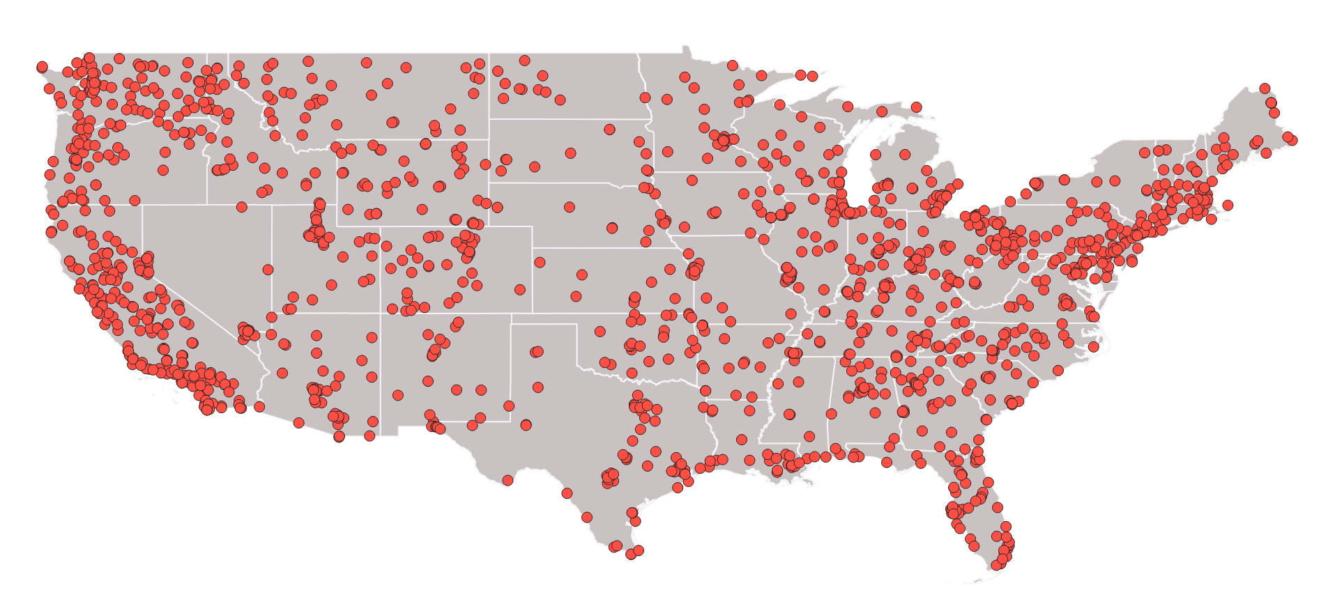
The base of the dataset we’re training on comes from the WildfireSpreadTS (WSTS) next-day wildfire spread benchmark. WSTS is a collection of 607 U.S. fire events (2018–2021), with data for each day the fire burned, with fields including fuel/vegetation, topography, current and forecasted weather, and landcover.
| Category | Source | Resolution | Feature |
|---|---|---|---|
| Vegetation | VIIRS | 375–750 m | VIIRS bands M11, I2, I1; NDVI; EVI2 |
| Weather | GridMET | 4 km | Total precipitation; Wind speed and direction; Min/Max temperature; Energy release component; Specific humidity; PDSI |
| Topography | USGS | 30 m | Slope; Aspect; Elevation; Landcover type |
| Forecast Weather | GFS | 28 km | Total precipitation; Wind speed and direction; Temperature; Specific humidity |
| Target | VIIRS | 375 m | Active fire |
WSTS improved upon prior datasets by adding multi-day time series inputs and higher temporal resolution paired with high spatial resolution. Our lab has further extended it with several additional years of fires, bringing the total to 1,067 events from 2016-2024.
Selecting the best source of PM 2.5 data is not a trivial task. There are many datasets available but they vary in the methods used to produce estimates, usually relying on a combination of physics based models, reanalysis, and satellite measurements of aerosol optical depth. Of these we evaluated four.
CAMS (Copernicus Atmosphere Monitoring Service) is a global, 3-hourly PM 2.5 forecast from the European Centre for Medium-Range Weather Forecasts that uses the IFS chemistry model, assimilates satellite aerosol optical depth, and reports PM 2.5 directly without sensor correction. MERRA-2 (NASA) is a global GOCART reanalysis where PM 2.5 is calculated from aerosol components; it does not use ground sensors directly. MERRA2R is the same dataset but bias-corrected against AirNow monitors to improve surface accuracy. NCAR (National Center for Atmospheric Research) provides a 12 km CONUS reanalysis using the WRF-CMAQ model that assimilates satellite AOD, designed for higher resolution U.S. air quality.
We tested each source by checking it’s accuracy relative to a PM 2.5 sensor reading dataset provided by AirNow.
The metrics we really care about are RMSE, which reflects overall accuracy, and slope, which shows how well the dataset scales as PM 2.5 concentrations increase. Because these datasets tend to under predict high PM 2.5 events, a slope closer to 1 means the dataset might better capture the high PM 2.5 coming from a fire.
| Source | Spearman | RMSE | Slope |
|---|---|---|---|
| NCAR | 0.475 | 20.600 | 1.336 |
| CAMS | 0.352 | 40.890 | 0.189 |
| MERRA2 | 0.426 | 54.019 | 0.166 |
| MERRA2R | 0.493 | 20.323 | 1.071 |
MERRA2R outperforms the others in all three metrics while being available globally from 2001-2024, and is what we will be using as a target variable for our training runs.
Training a model to predict fire spread is a binary semantic segmentation task, where the input is a multichannel raster made up of the WildfireSpreadTS dataset, the target is a binary mask of the next day’s burned pixels, and the output is a raster of probabilities that each pixel burned the next day. To train a model to predict PM 2.5 we will do something similar. Each input will be the same raster but with MERRA2R PM 2.5 added, and a mask of healthy / unhealthy PM 2.5 concentrations (over / under 80 ppm) as the target variable.
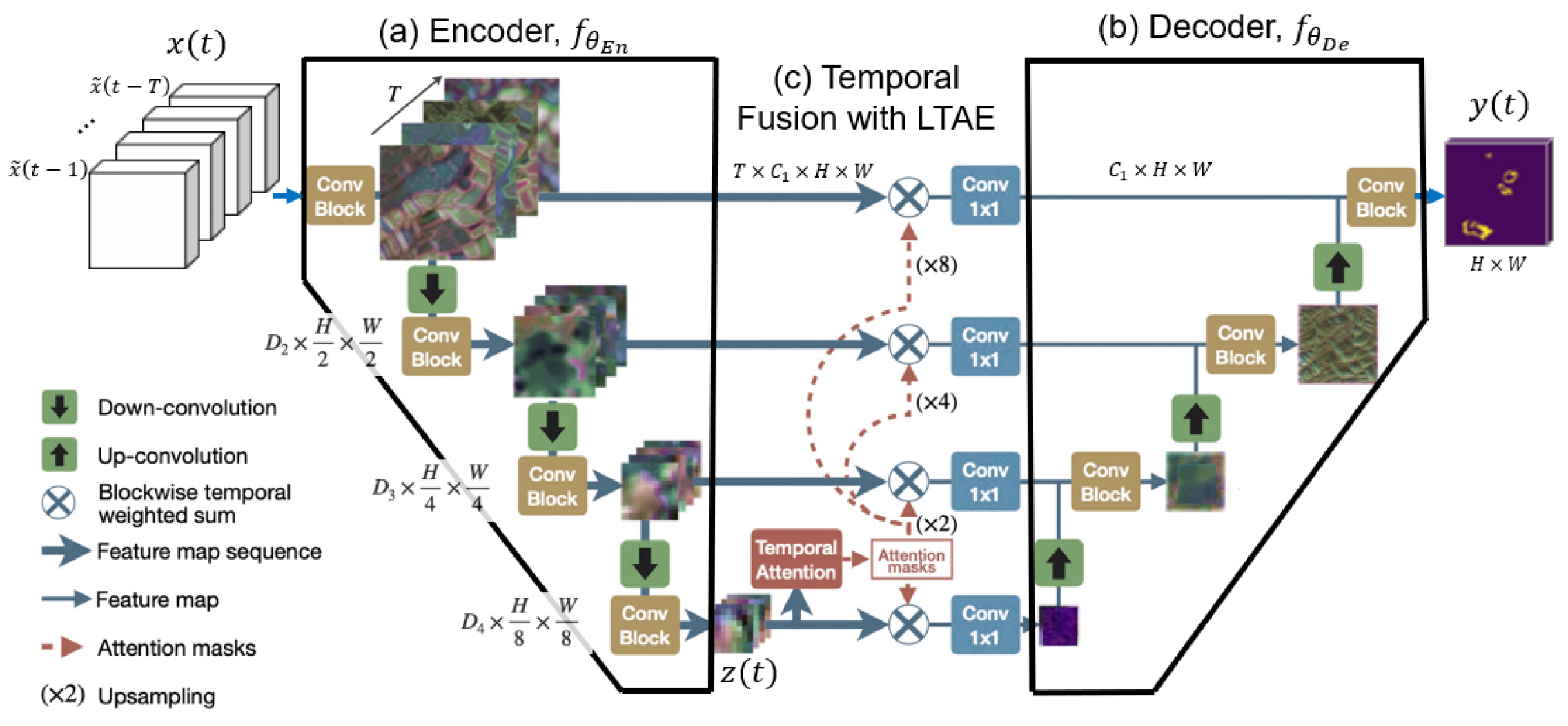
There are a few options for model architecture. Every architecture is a deep neural net that takes tensor representation of our raster as input, and does some sort of convolution on it, sometimes also using techniques like attention to take advantage of WSTS’s temporal component. Previous work has used U-Net, ConvLSTM, SwinUnet, and U-TAE architectures. We ended up using the U-TAE, which had performed the best on the original WildfireSpreadTS dataset.
We train with three loss functions designed for binary semantic segmentation. Binary Cross-Entropy (BCE) evaluates each pixel individually:
L_BCE = average over all pixels of [ -(y * log(ŷ) + (1 - y) * log(1 - ŷ)) ]
Jaccard Loss optimizes for overlap between predicted and true masks:
IoU = (intersection of prediction and ground truth) / (union of prediction and ground truth)
L_Jaccard = 1 - IoU
Dice Loss is similar to Jaccard but gives more weight to small regions:
DSC = (2 * intersection of prediction and ground truth) / (size of prediction + size of ground truth)
L_Dice = 1 - DSC
BCE focuses on per-pixel accuracy, while Jaccard and Dice better capture spatial overlap, which is useful for segmentation.
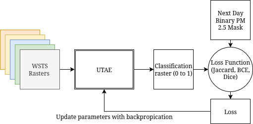
For training we make use of the setup found by previous modeling improvements by our lab. The previous five days of data are used as input, with dates encoded positionally. Our encoder is initialized with weights from pre-trained Res18 model and our decoder is trained from scratch. We use all three loss functions in a grid search. Our training split uses data from the year 2020 as a validation set, 2021 as test set, and the rest of the dataset for training.
Each model failed to converge to anything predictive, with average precision under 0.09 and flat loss curves. This may be due to several factors:
Future directions include expanding the spatial domain of the dataset to better capture full smoke plumes, incorporating covariates more directly relevant to PM 2.5 formation and transport, evaluating alternative PM 2.5 datasets with finer resolution or better integration with wildfire models, and including future burn area in model input. Additionally we’d also like to focus on predicting other harmful emissions more localized to the fire source.
← A Letter From My Grandfather https://lorn.us